A.16 The adi­a­batic the­o­rem

An adi­a­batic sys­tem is a sys­tem whose Hamil­ton­ian changes slowly in time. De­spite the time de­pen­dence of the Hamil­ton­ian, the wave func­tion can still be writ­ten in terms of the en­ergy eigen­func­tions $\psi_{\vec n}$ of the Hamil­ton­ian, be­cause the eigen­func­tions are com­plete. But since the Hamil­ton­ian changes with time, so do the en­ergy eigen­func­tions. And that af­fects how the co­ef­fi­cients of the eigen­func­tions evolve in time.

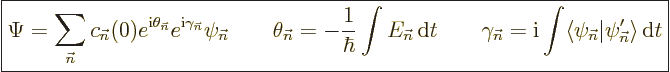
In par­tic­u­lar, in the adi­a­batic ap­prox­i­ma­tion, the wave func­tion of a sys­tem can be writ­ten as, {D.34}:

$$\fbox{$\displaystyle \Psi = \sum_{\vec n}c_{{\vec n}}(0) ... ...\langle\psi_{\vec n}\vert\psi_{\vec n}'\rangle{\,\rm d}t $} %$$ (A.74)

where the $c_{{\vec n}}(0)$ are con­stants. The an­gle $\theta_{\vec n}$ is called the “dy­namic phase” while the an­gle $\gamma_{\vec n}$ is called the “geo­met­ric phase.” Both phases are real. The prime on $\psi_{\vec n}$ in­di­cates the time de­riv­a­tive of the eigen­func­tion.

Note that if the Hamil­ton­ian does not de­pend on time, the above ex­pres­sion sim­pli­fies to the usual so­lu­tion of the Schrö­din­ger equa­tion as given in chap­ter 7.1.2. In par­tic­u­lar, in that case the geo­met­ric phase is zero and the dy­namic phase is the usual $-E_{{\vec n}}t$$\raisebox{.5pt}{$/$}$​$\hbar$.

Even if the Hamil­ton­ian de­pends on time, the geo­met­ric phase is still zero as long as the Hamil­ton­ian is real. The rea­son is that real Hamil­to­ni­ans have real eigen­func­tions; then $\gamma_{\vec n}$ can only be real, as it must be, if it is zero.

If the geo­met­ric phase is nonzero, you may be able to play games with it. Sup­pose first that Hamil­ton­ian changes with time be­cause some sin­gle pa­ra­me­ter $\lambda$ that it de­pends on changes with time. Then the geo­met­ric phase can be writ­ten as

$$\gamma_{\vec n}= {\rm i}\int \langle\psi_{\vec n}\vert \f... ...angle{\,\rm d}\lambda \equiv \int f(\lambda) {\,\rm d}\lambda$$

It fol­lows that if you bring the sys­tem back to the state it started out at, the to­tal geo­met­ric phase is zero, be­cause the lim­its of in­te­gra­tion will be equal.

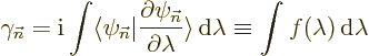
But now sup­pose that not one, but a set of pa­ra­me­ters $\vec\lambda$ $\vphantom0\raisebox{1.5pt}{$=$}$ $(\lambda_1,\lambda_2,\ldots)$ changes dur­ing the evo­lu­tion. Then the geo­met­ric phase is

$$\gamma_{\vec n}= {\rm i}\int \langle\psi_{\vec n}\vert\nab... ...+ f_2(\lambda_1,\lambda_2,\ldots) {\,\rm d}\lambda_2 + \ldots$$

and that is not nec­es­sar­ily zero when the sys­tem re­turns to the same state it started out at. In par­tic­u­lar, for two or three pa­ra­me­ters, you can im­me­di­ately see from the Stokes’ the­o­rem that the in­te­gral along a closed path will not nor­mally be zero un­less $\nabla_{\vec\lambda}\times\vec{f}$ $\vphantom0\raisebox{1.5pt}{$=$}$ 0. The geo­met­ric phase that an adi­a­batic sys­tem picks up dur­ing such a closed path is called “Berry’s phase.”

You might as­sume that it is ir­rel­e­vant since the phase of the wave func­tion is not ob­serv­able any­way. But if a beam of par­ti­cles is sent along two dif­fer­ent paths, the phase dif­fer­ence be­tween the paths will pro­duce in­ter­fer­ence ef­fects when the beams merge again.

Sys­tems that do not re­turn to the same state when they are taken around a closed loop are not just re­stricted to quan­tum me­chan­ics. A clas­si­cal ex­am­ple is the Fou­cault pen­du­lum, whose plane of os­cil­la­tion picks up a daily an­gu­lar de­vi­a­tion when the mo­tion of the earth car­ries it around a cir­cle. Such sys­tems are called “non­ho­lo­nomic” or an­ho­lo­nomic.