| Quantum Mechanics for Engineers |
|
© Leon van Dommelen |
|
Subsections
D.37 Forces by particle exchange derivations
D.37.1 Classical energy minimization
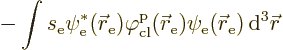
The energy minimization including a selecton is essentially the same
as the one for only spoton and foton field. That one has been
discussed in chapter A.22.1 and in detail in
{A.2}. So only the key differences will be listed here.
The energy to minimize is now
So the only real difference in the variational analysis is
That means that the Poisson equation now becomes
Since the Poisson equation is linear, the solution is 

 . Here
  is
the foton field (A.107) produced by the spoton as before, and
is
the foton field (A.107) produced by the spoton as before, and
 is a similar expression, but using the selecton
sarge and distance from the selecton:
is a similar expression, but using the selecton
sarge and distance from the selecton:
The energy lowering is now
Multiplying out, you get, of course, the energy lowerings for the
spoton and selecton in isolation. But you also get two additional
interaction terms between these sarges. These two terms are equal;
the selecton field evaluated at the position of
the spoton times spoton sarge is the same as the spoton field
at the selecton times selecton sarge. So it is
seen that each term contributes half to the Koulomb energy as claimed
in the text.
The foton field energy is still half of the particle-field interaction
energies and of opposite sign. That is why the energy change
is half of what you would expect from the interaction of the particles
with each other’s field: the other half is offset by changes in
field energy.
D.37.2 Quantum energy minimization
This derivation includes the selecton in the spoton-fotons system
analyzed in {A.22.3}. Since the analysis is essentially
unchanged, only the key differences will be highlighted.
If an selecton is added to the system, the system wave function
becomes
The demon can hold the selecton in its other hand. The Hamiltonian
will now of course include a term for the selecton in isolation, as
well as an interaction with the foton field. These are completely
analogous to the corresponding spoton terms.
So the energy to be minimized for the ground state becomes
If this is minimized as in {A.22.3}, the energy is
The square absolute value of a quantity can be found as the product of
that quantity times its complex conjugate. That gives the same energy
lowering as for the lone spoton, and a similar term for a lone
selecton. However, there is an additional term
If you write out the inner product integrals over the selecton
coordinates explicitly, this becomes
Summed over all  , the second term inside the square
brackets gives the same answer as the first; that is because opposite
values appear equally in the summation. Looking at the first
term, the summation over produces again the spoton potential
, the second term inside the square
brackets gives the same answer as the first; that is because opposite
values appear equally in the summation. Looking at the first
term, the summation over produces again the spoton potential
 , but now evaluated at the position
of the selecton. That then shows the additional energy lowering to be
, but now evaluated at the position
of the selecton. That then shows the additional energy lowering to be
Except for the differences in notation, that is the same
selecton-spoton interaction energy as found in {A.22.1}.
D.37.3 Rewriting the Lagrangian
The rules of engagement are as follows:
- The Cartesian axes are numbered using an index
 , with
1, 2, and 3 for
, with
1, 2, and 3 for  ,
,  , and
, and  respectively.
- Also,
 indicates the coordinate in the direction,
, , or .
indicates the coordinate in the direction,
, , or .
- Derivatives with respect to a coordinate are indicated by
a simple subscript .
- If the quantity being differentiated is a vector, a comma is
used to separate the vector index from differentiation ones.
- Index
 is the number immediately following in the
cyclic sequence ...123123...and
is the number immediately following in the
cyclic sequence ...123123...and  is the number
immediately preceding .
is the number
immediately preceding .
- If is already been used for something else,
 can be used
the same way.
can be used
the same way.
- Time derivatives are indicated by a subscript t.
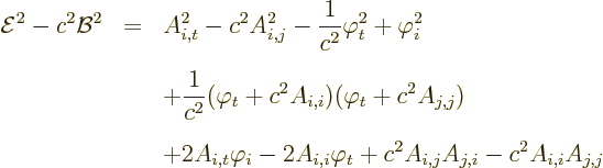
Consider first the square magnetic field:
Expanding out the square, that is equivalent to
The summation indices can now be cyclically redefined to give an
equivalent sum over equal to
The terms can be combined in sets of three as
Here summation over and is now understood.
The square electric field is
All together, that gives
as can be verified by multiplying out and simplifying.
The right hand side in the first line is the self-evident electromagnetic
Lagrangian density, except for the factor 
 2. The second
line is the square of the Lorentz condition quantity. The final line
can be written as a sum of pure derivatives:
2. The second
line is the square of the Lorentz condition quantity. The final line
can be written as a sum of pure derivatives:
Pure derivatives do not produce changes in the action, as the changes
in the potentials disappear on the boundaries of integration.
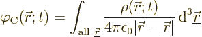
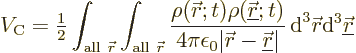
D.37.4 Coulomb potential energy
The Coulomb potential energy between charged particles is typically
derived in basic physics. But it can also easily be verified from the
conventional electromagnetic energy (A.143). In the steady
case, there is only the electric field, due to the Coulomb potential.
The energy may then be written as
where the first equality comes from the definition of the electric
field, the second from integration by parts and the third one from the
first Maxwell equation. Substitution of the Coulomb potential in
terms of the charge distribution as given in {A.22.8},
now gives the Koulomb potential energy  for a continuous
charge distribution:
for a continuous
charge distribution:
For point charges, the charge distribution is by definition
Here  is the three-dimensional delta function,
 the position of point charge , and
  its
charge.
its
charge.
Recall that the delta function picks out the value at from
whatever it is integrated against. Using this twice on the
Coulomb potential energy above,
That is the Coulomb potential energy for point charges.
Note again that physically all the energy is inside the
electromagnetic field. There is no energy of interaction of the
charged particles with the field. If equal charges move closer
together, they increase the energy in the electromagnetic field.
That requires work.