| Quantum Mechanics for Engineers |
|
© Leon van Dommelen |
|
Subsections
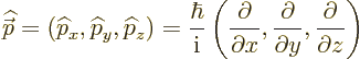
7.9 Position and Linear Momentum
The subsequent sections will be looking at the time evolution of
various quantum systems, as predicted by the Schrödinger equation.
However, before that can be done, first the eigenfunctions of position
and linear momentum must be found. That is something that the book
has been studiously avoiding so far. The problem is that the position
and linear momentum eigenfunctions have awkward issues with
normalizing them.
These normalization problems have consequences for the coefficients of
the eigenfunctions. In the orthodox interpretation, the square
magnitudes of the coefficients should give the probabilities of
getting the corresponding values of position and linear momentum. But
this statement will have to be modified a bit.
One good thing is that unlike the Hamiltonian, which is specific to a
given system, the position operator
and the linear momentum operator
are the same for all systems. So, you only need to find their
eigenfunctions once.
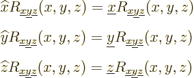
7.9.1 The position eigenfunction
The eigenfunction that corresponds to the particle being at a precise
 -position
  ,
,  -position
  , and
, and
 -position
  will be denoted by
  .
The eigenvalue problem is:
.
The eigenvalue problem is:
(Note the need in this analysis to use  for the
measurable particle position, since
for the
measurable particle position, since  are already used
for the eigenfunction arguments.)
are already used
for the eigenfunction arguments.)
To solve this eigenvalue problem, try again separation of variables, where it is assumed that
is of the form  .
Substitution gives the partial problem for
.
Substitution gives the partial problem for  as
as
This equation implies that at all points not equal to ,
 will have to be zero, otherwise there is no way that the two
sides can be equal. So, function can only be nonzero at the
single point . At that one point, it can be anything,
though.
will have to be zero, otherwise there is no way that the two
sides can be equal. So, function can only be nonzero at the
single point . At that one point, it can be anything,
though.
To resolve the ambiguity, the function is taken to be the
Dirac delta function,
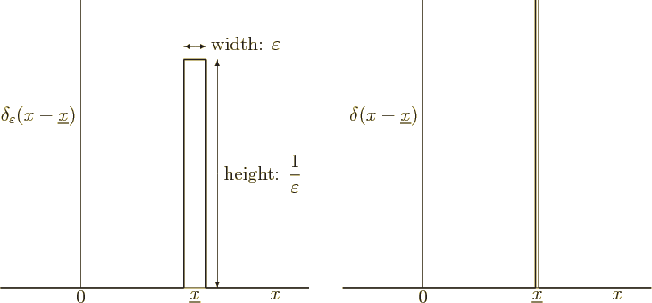
The delta function is, loosely speaking, sufficiently strongly infinite at
the single point  that its integral over that single point is
one. More precisely, the delta function is defined as the limiting
case of the function shown in the left hand side of figure
7.10.
that its integral over that single point is
one. More precisely, the delta function is defined as the limiting
case of the function shown in the left hand side of figure
7.10.
Figure 7.10:
Approximate Dirac delta function
 is shown left. The true
delta function
is shown left. The true
delta function  is the limit when
 becomes zero, and is an infinitely high,
infinitely thin spike, shown right. It is the eigenfunction
corresponding to a position
becomes zero, and is an infinitely high,
infinitely thin spike, shown right. It is the eigenfunction
corresponding to a position  .
.
 |
The fact that the integral is one leads to a very useful mathematical
property of delta functions: they are able to pick out one specific
value of any arbitrary given function  . Just take an
inner product of the delta function
. Just take an
inner product of the delta function  with .
It will produce the value of at the point , in other
words,
with .
It will produce the value of at the point , in other
words,  :
:
 |
(7.49) |
(Since the delta function is zero at all points except , it
does not make a difference whether or is used in the
integral.) This is sometimes called the “filtering property” of the delta function.
The problems for the position eigenfunctions  and
and  are the same
as the one for , and have a similar solution. The complete
eigenfunction corresponding to a measured position is
therefore:
are the same
as the one for , and have a similar solution. The complete
eigenfunction corresponding to a measured position is
therefore:
 |
(7.50) |
Here  is the three-dimensional delta function, a
spike at position
is the three-dimensional delta function, a
spike at position  whose volume integral equals one.
According to the orthodox interpretation, the probability of finding
the particle at for a given wave function  should be the square magnitude of the coefficient
  of the eigenfunction. This coefficient can be found as an inner
product:
of the eigenfunction. This coefficient can be found as an inner
product:
It can be simplified to
 |
(7.51) |
because of the property of the delta functions to pick out the
corresponding function value.
However, the apparent conclusion that 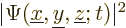 gives
the probability of finding the particle at is wrong.
The reason it fails is that eigenfunctions should be normalized; the
integral of their square should be one. The integral of the square of
a delta function is infinite, not one. That is OK, however;
gives
the probability of finding the particle at is wrong.
The reason it fails is that eigenfunctions should be normalized; the
integral of their square should be one. The integral of the square of
a delta function is infinite, not one. That is OK, however;  is
a continuously varying variable, and the chances of finding the
particle at to an infinite number of digits
accurate would be zero. So, the properly normalized eigenfunctions
would have been useless anyway.
is
a continuously varying variable, and the chances of finding the
particle at to an infinite number of digits
accurate would be zero. So, the properly normalized eigenfunctions
would have been useless anyway.
Instead, according to Born's statistical interpretation of chapter
3.1, the expression
gives the probability of finding the particle in an infinitesimal
volume  around . In other words,
 gives the probability of finding the particle
near location per unit volume. (The underlines below the position coordinates
are no longer needed to avoid ambiguity and have been dropped.)
gives the probability of finding the particle
near location per unit volume. (The underlines below the position coordinates
are no longer needed to avoid ambiguity and have been dropped.)
Besides the normalization issue, another idea that needs to be
somewhat modified is a strict collapse of the wave function. Any
position measurement that can be done will leave some uncertainty
about the precise location of the particle: it will leave
 nonzero over a small range of positions, rather than
just one position. Moreover, unlike energy eigenstates, position
eigenstates are not stationary: after a position measurement,
will again spread out as time increases.
nonzero over a small range of positions, rather than
just one position. Moreover, unlike energy eigenstates, position
eigenstates are not stationary: after a position measurement,
will again spread out as time increases.
Key Points

- Position eigenfunctions are delta functions.
-
- They are not properly normalized.
-
- The coefficient of the position eigenfunction for a position
is the good old wave function .
-
- Because of the fact that the delta functions are not normalized,
the square magnitude of does not give the
probability that the particle is at position .
-
- Instead the square magnitude of gives the
probability that the particle is near position per unit
volume.
-
- Position eigenfunctions are not stationary, so localized
particle wave functions will spread out over time.
7.9.2 The linear momentum eigenfunction
Turning now to linear momentum, the eigenfunction that corresponds to
a precise linear momentum  will be indicated as
 . If you again assume that this
eigenfunction is of the form , the partial problem for is found to be:
. If you again assume that this
eigenfunction is of the form , the partial problem for is found to be:
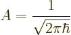
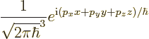
The solution is a complex exponential:
where  is a constant.
Just like the position eigenfunction earlier, the linear momentum
eigenfunction has a normalization problem. In particular, since it
does not become small at large  , the integral of its square
is infinite, not one. The solution is to ignore the problem and to
just take a nonzero value for ; the choice that works out
best is to take:
, the integral of its square
is infinite, not one. The solution is to ignore the problem and to
just take a nonzero value for ; the choice that works out
best is to take:
(However, other books, in particular nonquantum ones, are likely to
make a different choice.)
The problems for the and linear momenta have similar
solutions, so the full eigenfunction for linear momentum takes the
form:
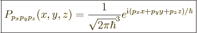 |
(7.52) |
The coefficient  of the momentum eigenfunction is
very important in quantum analysis. It is indicated by the special
symbol
of the momentum eigenfunction is
very important in quantum analysis. It is indicated by the special
symbol  and called the “momentum space wave function.” Like all coefficients, it can be
found by taking an inner product of the eigenfunction with the wave
function:
and called the “momentum space wave function.” Like all coefficients, it can be
found by taking an inner product of the eigenfunction with the wave
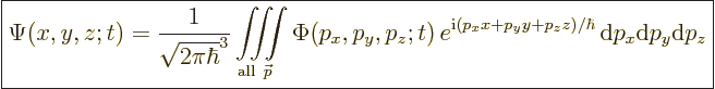
function:
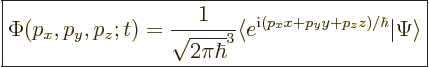 |
(7.53) |
The momentum space wave function does not quite give the probability
for the momentum to be . Instead it turns out
that
gives the probability of finding the linear momentum within a small
momentum range  around
. In other words,
around
. In other words, 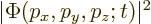 gives the probability of finding the particle with a momentum near
per unit
gives the probability of finding the particle with a momentum near
per unit momentum space volume.
That
is much like the square magnitude of the normal
wave function gives the probability of finding the particle near
location per unit physical volume. The momentum space wave
function  is in the momentum space what the
normal wave function is in the physical space .
is in the momentum space what the
normal wave function is in the physical space .
There is even an inverse relationship to recover from
, and it is easy to remember:
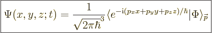 |
(7.54) |
where the subscript on the inner product indicates that the
integration is over momentum space rather than physical space.
If this inner product is written out, it reads:
 |
(7.55) |
Mathematicians prove this formula under the name “Fourier
Inversion Theorem”, {A.26}. But it really is
just the same sort of idea as writing as a sum of
eigenfunctions  times their coefficients
  , as in
 . In this case, the coefficients
are given by and the eigenfunctions by the exponential
(7.52). The only real difference is that the sum has become
an integral since
. In this case, the coefficients
are given by and the eigenfunctions by the exponential
(7.52). The only real difference is that the sum has become
an integral since  has continuous values, not discrete ones.
Key Points
-
- The linear momentum eigenfunctions are complex exponentials
of the form:
-
- They are not properly normalized.
-
- The coefficient of the linear momentum eigenfunction for a
momentum is indicated by
. It is called the momentum space wave
function.
-
- Because of the fact that the momentum eigenfunctions are not
normalized, the square magnitude of does not
give the probability that the particle has momentum
.
-
- Instead the square magnitude of gives the
probability that the particle has a momentum close to
per unit momentum space volume.
-
- In writing the complete wave function in terms of the momentum
eigenfunctions, you must integrate over the momentum instead of sum.
-
- The transformation between the physical space wave function
and the momentum space wave function is called the
Fourier transform. It is invertible.