D.39 Se­lec­tion rules

This note de­rives the se­lec­tion rules for elec­tric di­pole tran­si­tions be­tween two hy­dro­gen states $\psi_{\rm {L}}$ and $\psi_{\rm {H}}$. Some se­lec­tion rules for for­bid­den tran­si­tions are also de­rived. The de­riva­tions for for­bid­den tran­si­tions use some more ad­vanced re­sults from later chap­ters. It may be noted that in any case, the Hamil­ton­ian as­sumes that the ve­loc­ity of the elec­trons is small com­pared to the speed of light.

Ac­cord­ing to chap­ter 4.3, the hy­dro­gen states take the form $\psi_{\rm {L}}$ $\vphantom0\raisebox{1.5pt}{$=$}$ $\psi_{n_{\rm {L}}l_{\rm {L}}m_{\rm {L}}}{\updownarrow}$ and $\psi_{\rm {H}}$ $\vphantom0\raisebox{1.5pt}{$=$}$ $\psi_{n_{\rm {H}}l_{\rm {H}}m_{\rm {H}}}{\updownarrow}$. Here 1 $\raisebox{-.3pt}{$\leqslant$}$ $n$, 0 $\raisebox{-.3pt}{$\leqslant$}$ $l$ $\raisebox{-.3pt}{$\leqslant$}$ $n$ and $\vert m\vert$ $\raisebox{-.3pt}{$\leqslant$}$ $l$ are in­te­ger quan­tum num­bers. The fi­nal ${\updownarrow}$ rep­re­sents the elec­tron spin state, up or down.

As noted in the text, al­lowed elec­tric di­pole tran­si­tions must re­spond to at least one com­po­nent of a con­stant am­bi­ent elec­tric field. That means that they must have a nonzero value for at least one elec­tri­cal di­pole mo­ment,

$$\langle \psi_{\rm {L}}\vert r_i\vert\psi_{\rm {H}}\rangle \ne 0$$

where $r_i$ can be one of $r_1$ $\vphantom0\raisebox{1.5pt}{$=$}$ $x$, $r_2$ $\vphantom0\raisebox{1.5pt}{$=$}$ $y$, or $r_3$ $\vphantom0\raisebox{1.5pt}{$=$}$ $z$ for the three dif­fer­ent com­po­nents of the elec­tric field.

The trick in iden­ti­fy­ing when these in­ner prod­ucts are zero is based on tak­ing in­ner prod­ucts with clev­erly cho­sen com­mu­ta­tors. Since the hy­dro­gen states are eigen­func­tions of $\L _z$, the fol­low­ing com­mu­ta­tor is use­ful

$$\langle \psi_{\rm {L}}\vert [r_i,\L _z]\vert\psi_{\rm {H}}\... ..._{\rm {L}}\vert r_i\L _z - \L _zr_i \vert\psi_{\rm {H}}\rangle$$

For the $r_i\L _z$ term in the right hand side, the op­er­a­tor $\L _z$ acts on $\psi_{\rm {H}}$ and pro­duces a fac­tor $m_{\rm {H}}\hbar$, while for the $\L _zr_i$ term, $\L _z$ can be taken to the other side of the in­ner prod­uct and then acts on $\psi_{\rm {L}}$, pro­duc­ing a fac­tor $m_{\rm {L}}\hbar$. So:

$$\langle \psi_{\rm {L}}\vert [r_i,\L _z]\vert\psi_{\rm {H}}\... ...ar \langle\psi_{\rm {L}}\vert r_i\vert\psi_{\rm {H}}\rangle %$$ (D.24)

The fi­nal in­ner prod­uct is the di­pole mo­ment of in­ter­est. There­fore, if a suit­able ex­pres­sion for the com­mu­ta­tor in the left hand side can be found, it will fix the di­pole mo­ment.

In par­tic­u­lar, ac­cord­ing to chap­ter 4.5.4 $[z,\L _z]$ is zero. That means ac­cord­ing to equa­tion (D.24) above that the di­pole mo­ment $\langle\psi_{\rm {L}}\vert z\vert\psi_{\rm {H}}\rangle$ in the right hand side will have to be zero too, un­less $m_{\rm {H}}$ $\vphantom0\raisebox{1.5pt}{$=$}$ $m_{\rm {L}}$. So the first con­clu­sion is that the $z$-​com­po­nent of the elec­tric field does not do any­thing un­less $m_{\rm {H}}$ $\vphantom0\raisebox{1.5pt}{$=$}$ $m_{\rm {L}}$. One down, two to go.

For the $x$ and $y$ com­po­nents, from chap­ter 4.5.4

$$[x,\L _z]= -{\rm i}\hbar y \qquad [y,\L _z] = {\rm i}\hbar x$$

Plug­ging that into (D.24) pro­duces

$$- {\rm i}\hbar \langle\psi_{\rm {L}}\vert y\vert\psi_{\rm {... ...})\hbar \langle\psi_{\rm {L}}\vert y\vert\psi_{\rm {H}}\rangle$$

From these equa­tions it is seen that the $y$ di­pole mo­ment is zero if the $x$ one is, and vice-versa. Fur­ther, plug­ging the $y$ di­pole mo­ment from the first equa­tion into the sec­ond pro­duces

$${\rm i}\hbar \langle\psi_{\rm {L}}\vert x\vert\psi_{\rm {H}... ...\hbar} \langle\psi_{\rm {L}}\vert x\vert\psi_{\rm {H}}\rangle$$

and if the $x$ di­pole mo­ment is nonzero, that re­quires that $(m_{\rm {H}}-m_{\rm {L}})^2$ is one, so $m_{\rm {H}}$ $\vphantom0\raisebox{1.5pt}{$=$}$ $m_{\rm {L}}\pm1$. It fol­lows that di­pole tran­si­tions can only oc­cur if $m_{\rm {H}}$ $\vphantom0\raisebox{1.5pt}{$=$}$ $m_{\rm {L}}$, through the $z$ com­po­nent of the elec­tric field, or if $m_{\rm {H}}$ $\vphantom0\raisebox{1.5pt}{$=$}$ $m_{\rm {L}}\pm1$, through the $x$ and $y$ com­po­nents.

To de­rive se­lec­tion rules in­volv­ing the az­imuthal quan­tum num­bers $l_{\rm {H}}$ and $l_{\rm {L}}$, the ob­vi­ous ap­proach would be to try the com­mu­ta­tor $[r_i,\L ^2]$ since $\L ^2$ pro­duces $l(l+1)\hbar^2$. How­ever, ac­cord­ing to chap­ter 4.5.4, (4.68), this com­mu­ta­tor will bring in the ${\skew 2\widehat{\skew{-1}\vec r}}$ $\times$ ${\skew 4\widehat{\vec L}}$ op­er­a­tor, which can­not be han­dled. The com­mu­ta­tor that works is the sec­ond of (4.73):

$$[[r_i,\L ^2],\L ^2] = 2\hbar^2(r_i\L ^2+\L ^2r_i)$$

where by the de­f­i­n­i­tion of the com­mu­ta­tor

$$[[r_i,\L ^2],\L ^2] = (r_i\L ^2-\L ^2r_i)\L ^2 - \L ^2(r_i\L ^2-\L ^2r_i) = r_i\L ^2\L ^2-2\L ^2r_i\L ^2+\L ^2\L ^2r_i$$

Eval­u­at­ing $\langle\psi_{\rm {L}}\vert[[r_i,\L ^2],\L ^2]\vert\psi_{\rm {H}}\rangle$ ac­cord­ing to each of the two equa­tions above and equat­ing the re­sults gives

$$2\hbar^2[l_{\rm {H}}(l_{\rm {H}}+1)+l_{\rm {L}}(l_{\rm {L}}... ...)]^2 \langle\psi_{\rm {L}}\vert r_i\vert\psi_{\rm {H}}\rangle$$

For $\langle\psi_{\rm {L}}\vert r_i\vert\psi_{\rm {H}}\rangle$ to be nonzero, the nu­mer­i­cal fac­tors in the left and right hand sides must be equal,

$$2 [l_{\rm {H}}(l_{\rm {H}}+1)+l_{\rm {L}}(l_{\rm {L}}+1)] = [l_{\rm {H}}(l_{\rm {H}}+1)-l_{\rm {L}}(l_{\rm {L}}+1)]^2$$

The right hand side is ob­vi­ously zero for $l_{\rm {H}}$ $\vphantom0\raisebox{1.5pt}{$=$}$ $l_{\rm {L}}$, so $l_{\rm {H}}-l_{\rm {L}}$ can be fac­tored out of it as

$$[l_{\rm {H}}(l_{\rm {H}}+1)-l_{\rm {L}}(l_{\rm {L}}+1)]^2 = (l_{\rm {H}}-l_{\rm {L}})^2(l_{\rm {H}}+l_{\rm {L}}+1)^2$$

and the left hand side can be writ­ten in terms of these same fac­tors as

$$2 [l_{\rm {H}}(l_{\rm {H}}+1)+l_{\rm {L}}(l_{\rm {L}}+1)] = (l_{\rm {H}}-l_{\rm {L}})^2 + (l_{\rm {H}}+l_{\rm {L}}+1)^2 - 1$$

Equat­ing the two re­sults and sim­pli­fy­ing gives

$$[(l_{\rm {H}}-l_{\rm {L}})^2-1][(l_{\rm {H}}+l_{\rm {L}}+1)^2-1] = 0$$

The sec­ond fac­tor is only zero if $l_{\rm {H}}$ $\vphantom0\raisebox{1.5pt}{$=$}$ $l_{\rm {L}}$ $\vphantom0\raisebox{1.5pt}{$=$}$ 0, but then $\langle\psi_{\rm {L}}\vert r_i\vert\psi_{\rm {H}}\rangle$ is still zero be­cause both states are spher­i­cally sym­met­ric. It fol­lows that the first fac­tor will have to be zero for di­pole tran­si­tions to be pos­si­ble, and that means that $l_{\rm {H}}$ $\vphantom0\raisebox{1.5pt}{$=$}$ $l_{\rm {L}}\pm1$.

The spin is not af­fected by the per­tur­ba­tion Hamil­ton­ian, so the di­pole mo­ment in­ner prod­ucts are still zero un­less the spin mag­netic quan­tum num­bers $m_s$ are the same, both spin-up or both spin-down. In­deed, if the elec­tron spin is not af­fected by the elec­tric field to the ap­prox­i­ma­tions made, then ob­vi­ously it can­not change. That com­pletes the se­lec­tion rules as given in chap­ter 7.4.4 for elec­tric di­pole tran­si­tions.

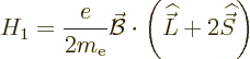
Now con­sider the ef­fect of the mag­netic field on tran­si­tions. For such tran­si­tions to be pos­si­ble, the ma­trix el­e­ment formed with the mag­netic field must be nonzero. Like the elec­tric field, the mag­netic field can be ap­prox­i­mated as spa­tially con­stant and quasi-steady. The per­tur­ba­tion Hamil­ton­ian of a con­stant mag­netic field is ac­cord­ing to chap­ter 13.4

$$H_1 = \frac{e}{2m_{\rm e}} \skew2\vec{\cal B}\cdot \left({\skew 4\widehat{\vec L}}+ 2 {\skew 6\widehat{\vec S}}\right)$$

Note that now elec­tron spin must be in­cluded in the dis­cus­sion.

Ac­cord­ing to this per­tur­ba­tion Hamil­ton­ian, the per­tur­ba­tion co­ef­fi­cient $H_{\rm {HL}}$ for the $z$-​com­po­nent of the mag­netic field is pro­por­tional to

$$\langle \psi_{\rm {L}}\vert\L _z+2{\widehat S}_z\vert\psi_{\rm {H}}\rangle$$

and that is zero be­cause $\psi_{\rm {H}}{\updownarrow}$ is an eigen­func­tion of both op­er­a­tors and or­thog­o­nal to $\psi_{\rm {L}}{\updownarrow}$. So the $z$-​com­po­nent of the mag­netic field does not pro­duce tran­si­tions to dif­fer­ent states.

How­ever, the $x$-​com­po­nent (and sim­i­larly the $y$-​com­po­nent) pro­duces a per­tur­ba­tion co­ef­fi­cient pro­por­tional to

$$\langle \psi_{\rm {L}}\vert\L _x\vert\psi_{\rm {H}}\rangle ... ...le \psi_{\rm {L}}\vert{\widehat S}_x\vert\psi_{\rm {H}}\rangle$$

Ac­cord­ing to chap­ter 12.11, the ef­fect of $\L _x$ on a state with mag­netic quan­tum num­ber $m_{\rm {H}}$ is to turn it into a lin­ear com­bi­na­tion of two sim­i­lar states with mag­netic quan­tum num­bers $m_{\rm {H}}+1$ and $m_{\rm {H}}-1$. There­fore, for the first in­ner prod­uct above to be nonzero, $m_{\rm {L}}$ will have to be ei­ther $m_{\rm {H}}+1$ or $m_{\rm {H}}-1$. Also the or­bital az­imuthal mo­men­tum num­bers $l$ will need to be the same, and so will the spin mag­netic quan­tum num­bers $m_s$. And the prin­ci­pal quan­tum num­bers $n$, for that mat­ter; oth­er­wise the ra­dial parts of the wave fuc­tions are or­thog­o­nal.

The mag­netic field sim­ply wants to ro­tate the or­bital an­gu­lar mo­men­tum vec­tor in the hy­dro­gen atom. That does not change the en­ergy, in the ab­sence of an av­er­age am­bi­ent mag­netic field. For the sec­ond in­ner prod­uct, the spin mag­netic quan­tum num­bers have to be dif­fer­ent by one unit, while the or­bital mag­netic quan­tum num­bers must now be equal. So, all to­gether

$$l_{\rm {H}} = l_{\rm {L}} \qquad m_{\rm {H}} = m_{\rm {L}}... ...{\rm {H}}} = m_{s,{\rm {L}}} \mbox{ or } m_{s,{\rm {L}}} \pm 1$$

and ei­ther the or­bital or the spin mag­netic quan­tum num­bers must be un­equal. That are the se­lec­tion rules as given in chap­ter 7.4.4 for mag­netic di­pole tran­si­tions. Since the en­ergy does not change in these tran­si­tions, Fermi’s golden rule would have the de­cay rate zero. Fermi’s analy­sis is not ex­act, but such tran­si­tions should be very rare.

The log­i­cal way to pro­ceed to elec­tric quadru­pole tran­si­tions would be to ex­pand the elec­tric field in a Tay­lor se­ries in terms of $y$:

$$\skew3\vec{\cal E}= {\hat k}{\cal E}_{\rm {f}} \cos\Big(\om... ...}\frac{\omega}{c} {\cal E}_{\rm {f}} \sin(\omega t - \alpha) y$$

The first term is the con­stant elec­tric field of the elec­tric di­pole ap­prox­i­ma­tion, and the sec­ond would then give the elec­tric quadru­pole ap­prox­i­ma­tion. How­ever, an elec­tric field in which ${\cal E}_z$ is a mul­ti­ple of $y$ is not con­ser­v­a­tive, so the elec­tro­sta­tic po­ten­tial does no longer ex­ist.

It is nec­es­sary to re­treat to the so-called vec­tor po­ten­tial $\skew3\vec A$. It is then sim­plest to chose this po­ten­tial to get rid of the elec­tro­sta­tic po­ten­tial al­to­gether. In that case the typ­i­cal elec­tro­mag­netic wave is de­scribed by the vec­tor po­ten­tial

$$\skew3\vec A = - {\hat k}\frac{1}{\omega} {\cal E}_{\rm {f... ...rtial t} \quad \skew2\vec{\cal B}= \nabla \times \skew3\vec A$$

In terms of the vec­tor po­ten­tial, the per­tur­ba­tion Hamil­ton­ian is, chap­ter 13.1 and 13.4, and as­sum­ing a weak field,

$$H_1 = \frac{e}{2m_{\rm e}} (\skew3\vec A\cdot{\skew 4\wideh... ...{e}{m_{\rm e}}{\skew 6\widehat{\vec S}}\cdot\skew2\vec{\cal B}$$

Ig­nor­ing the spa­tial vari­a­tion of $\skew3\vec A$, this ex­pres­sion pro­duces an Hamil­ton­ian co­ef­fi­cient

$$H_{\rm {HL}} = - \frac{e}{m_{\rm e}\omega} {\cal E}_{\rm {f... ...le \psi_{\rm {L}}\vert{\widehat p}_z\vert\psi_{\rm {H}}\rangle$$

That should be same as for the elec­tric di­pole ap­prox­i­ma­tion, since the field is now com­pletely de­scribed by $\skew3\vec A$, but it is not quite. The ear­lier de­riva­tion as­sumed that the elec­tric field is quasi-steady. How­ever, ${\widehat p}_z$ is equal to the com­mu­ta­tor ${{\rm i}}m_{\rm e}[H_0,z]$$\raisebox{.5pt}{$/$}$​$\hbar$ where $H_0$ is the un­per­turbed hy­dro­gen atom Hamil­ton­ian. If that is plugged in and ex­panded, it is found that the ex­pres­sions are equiv­a­lent, pro­vided that the per­tur­ba­tion fre­quency is close to the fre­quency of the pho­ton re­leased in the tran­si­tion, and that that fre­quency is suf­fi­ciently rapid that the phase shift from sine to co­sine can be ig­nored. Those are in fact the nor­mal con­di­tions.

Now con­sider the sec­ond term in the Tay­lor se­ries of $\skew3\vec A$ with re­spect to $y$. It pro­duces a per­tur­ba­tion Hamil­ton­ian

$$\frac{e}{m_{\rm e}}\frac{1}{c}{\cal E}_{\rm {f}}\cos(\omega t-\alpha) y {\widehat p}_z$$

The fac­tor $y{\widehat p}_z$ can be triv­ially rewrit­ten to give

$$\frac{e}{2m_{\rm e}}\frac{1}{c}{\cal E}_{\rm {f}}\cos(\omeg... ...\rm {f}}\cos(\omega t-\alpha)(y{\widehat p}_z+z{\widehat p}_y)$$

The first term has al­ready been ac­counted for in the mag­netic di­pole tran­si­tions dis­cussed above, be­cause the fac­tor within paren­the­ses is $\L _x$. The sec­ond term is the elec­tric quadru­pole Hamil­ton­ian for the con­sid­ered wave.

As sec­ond terms in the Tay­lor se­ries, both Hamil­to­ni­ans will be much smaller than the elec­tric di­pole one. The fac­tor that they are smaller can be es­ti­mated from com­par­ing the first and sec­ond term in the Tay­lor se­ries. Note that $c$$\raisebox{.5pt}{$/$}$​$\omega$ is pro­por­tional to the wave length $\lambda$ of the elec­tro­mag­netic wave. Also, the ad­di­tional po­si­tion co­or­di­nate in the op­er­a­tor scales with the atom size, call it $R$. So the fac­tor that the mag­netic di­pole and elec­tric quadru­pole ma­trix el­e­ments are smaller than the elec­tric di­pole one is $R$$\raisebox{.5pt}{$/$}$​$\lambda$. Since tran­si­tion prob­a­bil­i­ties are pro­por­tional to the square of the cor­re­spond­ing ma­trix el­e­ment, it fol­lows that, all else be­ing the same, mag­netic di­pole and elec­tric quadru­pole tran­si­tions are slower than elec­tric di­pole ones by a fac­tor $(R/\lambda)^2$. (But note the ear­lier re­mark on the prob­lem for the hy­dro­gen atom that the en­ergy does not change in mag­netic di­pole tran­si­tions.)

The se­lec­tion rules for the elec­tric quadru­pole Hamil­ton­ian can be nar­rowed down with a bit of sim­ple rea­son­ing. First, since the hy­dro­gen eigen­func­tions are com­plete, ap­ply­ing any op­er­a­tor on an eigen­func­tion will al­ways pro­duce a lin­ear com­bi­na­tion of eigen­func­tions. Now re­con­sider the de­riva­tion of the elec­tric di­pole se­lec­tion rules above from that point of view. It is then seen that $z$ only pro­duces eigen­func­tions with the same val­ues of $m$ and the val­ues of $l$ ex­actly one unit dif­fer­ent. The op­er­a­tors $x$ and $y$ change both $m$ and $l$ by ex­actly one unit. And the com­po­nents of lin­ear mo­men­tum do the same as the cor­re­spond­ing com­po­nents of po­si­tion, since ${\widehat p}_i$ $\vphantom0\raisebox{1.5pt}{$=$}$ ${{\rm i}}m_{\rm e}[H_0,r_i]$$\raisebox{.5pt}{$/$}$​$\hbar$ and $H_0$ does not change the eigen­func­tions, just their co­ef­fi­cients. There­fore $y{\widehat p}_z+z{\widehat p}_y$ pro­duces only eigen­func­tions with az­imuthal quan­tum num­ber $l$ ei­ther equal to $l_{\rm {H}}$ or to $l_{\rm {H}}\pm2$, de­pend­ing on whether the two unit changes re­in­force or can­cel each other. Fur­ther­more, it pro­duces only eigen­func­tions with $m$ equal to $m_{\rm {H}}\pm1$. How­ever, $x{\widehat p}_y+y{\widehat p}_x$, cor­re­spond­ing to a wave along an­other axis, will pro­duce val­ues of $m$ equal to $m_{\rm {H}}$ or to $m_{\rm {H}}\pm2$. There­fore the se­lec­tion rules be­come:

$$l_{\rm {H}} = l_{\rm {L}} \mbox{ or } l_{\rm {L}} \pm 2 \q... ... } m_{\rm {L}} \pm 2 \qquad m_{s,{\rm {H}}} = m_{s,{\rm {L}}}$$

That are the se­lec­tion rules as given in chap­ter 7.4.4 for elec­tric quadru­pole tran­si­tions. These ar­gu­ments ap­ply equally well to the mag­netic di­pole tran­si­tion, but there the pos­si­bil­i­ties are nar­rowed down much fur­ther be­cause the an­gu­lar mo­men­tum op­er­a­tors only pro­duce a cou­ple of eigen­func­tions. It may be noted that in ad­di­tion, elec­tric quadru­pole tran­si­tions from $l_{\rm {H}}$ $\vphantom0\raisebox{1.5pt}{$=$}$ 0 to $l_{\rm {L}}$ $\vphantom0\raisebox{1.5pt}{$=$}$ 0 are not pos­si­ble be­cause of spher­i­cal sym­me­try.